Introduction to Machine Learning with Julia
The Julia language was originally released in 2012 by Alan Edelman, Stefan Karpinski, Jeff Bezanson, and Viral Shah. Its popularity has been increasing exponentially in the last few years and its speed and community have been key. Furthermore, and taking the words of Ben Lauwens in its book Think Julia the reasons for picking up Julia are: Julia is developed as a high-performance programming language.
- Julia uses multiple dispatches, which allows the programmer to choose from different programming patterns adapted to the application.
- Julia is a dynamically typed language that can easily be used interactively.
- Julia has a nice high-level syntax that is easy to learn.
- Julia is an optionally typed programming language whose (user-defined) data types make the code clearer and more robust.
Being you an R user, Python user or even not proficient with any machine learning related language, this guide is aimed to give you a hand understanding julia and how it is applied to ML.
Getting Started
So first of all, the packages we are using today for the classification task is MLJ package. DataFrames and CSV are for data handling and StatsPlots for visualization.
NOTE: The using term is used to import packages.
If you do not have them installed you should run using Pkg;Pkg.add(“packageName”).
using MLJ
using CSV
using DataFrames
using StatsPlots
using Random
Now we need to load the data we are testing, we will be using the data from UCI repository, namely the Breast Cancer Coimbra Data Set. We will import and make an initial analysis of the data present, by viewing scitypes selected, and the schema and take a glimpse at the first four records of the data.
Data Import and visualizations
Let’s download the data and put the path to it in the CSV.read(<path>).
data = CSV.read("dataR2.csv");
@show schema(data).scitypes
@show schema(data)
first(data, 4)

Our purpose for today is to create models that can predict the Classification variable. Which is the classification of the patient.
- 1 is for healthy controls
- 2 is for real patient
To predict it, we will use the remaining variables (like Age, BMI, etc). So we will check how the variable is distributed in the dataset to see if it is balanced.
by(data,:Classification,nrow)
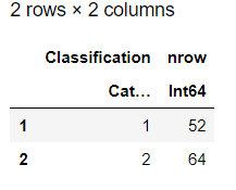
Fairly balanced, so let’s look at some descriptive statistics of the whole dataset.
describe(data)
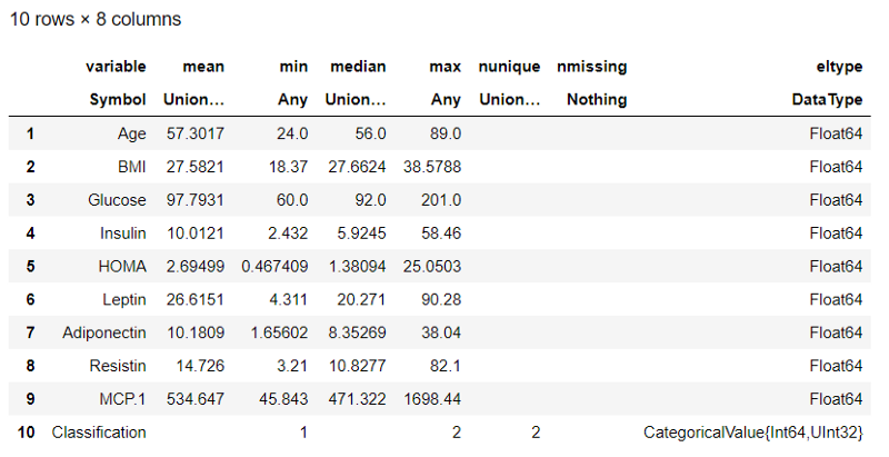
No missings and all numeric data. That’s cool! For MLJ package, scitypes are core. So we will coerce them to continuous and OrderedFactor to apply the most known models down the line.
coerce!(data, :Classification=>OrderedFactor);
coerce!(data, Count=>Continuous);
Now we are ready to make some visualizations and get a better understanding of the data at hand.
data_m=convert(Matrix,data)
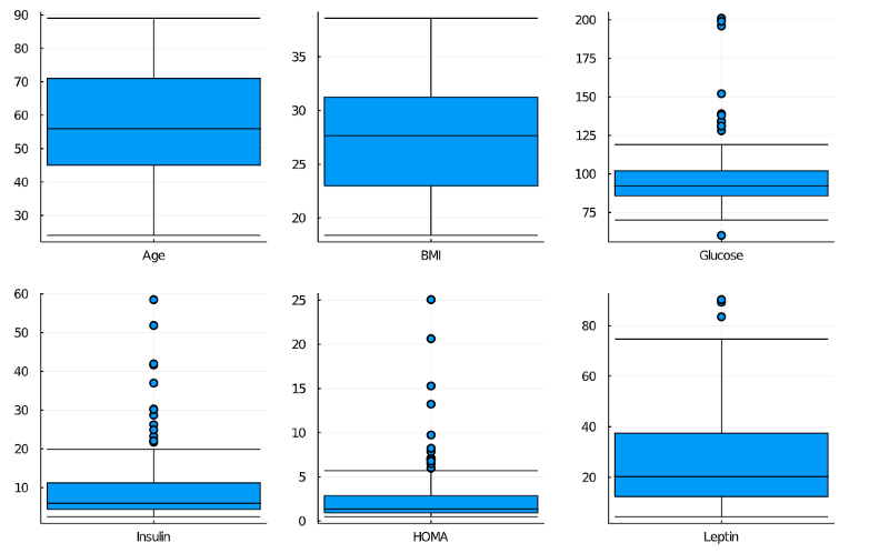
p=boxplot(layout=9)
p=boxplot(layout=9,size=(800,800))
for i in 1:9
    boxplot!([names(data)[i]],data_m[:,i], subplot = i,label=nothing )
end
display(p)

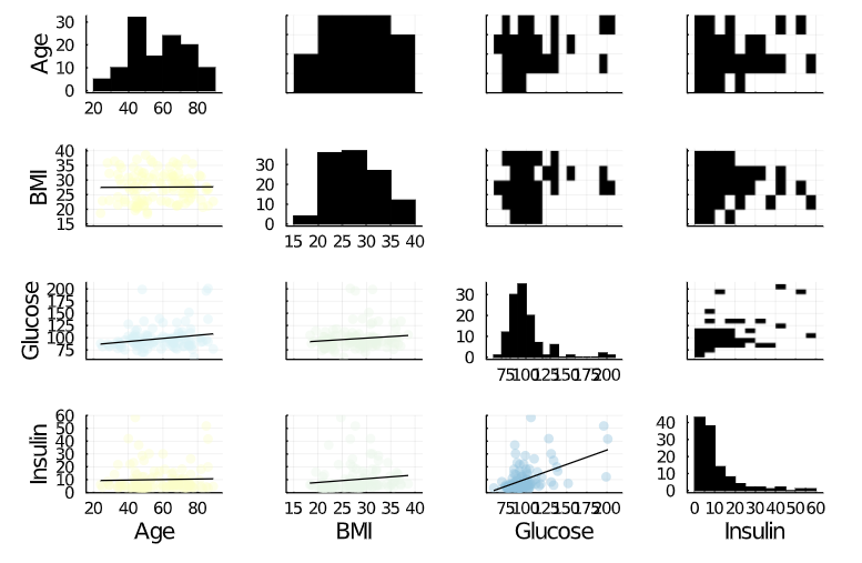
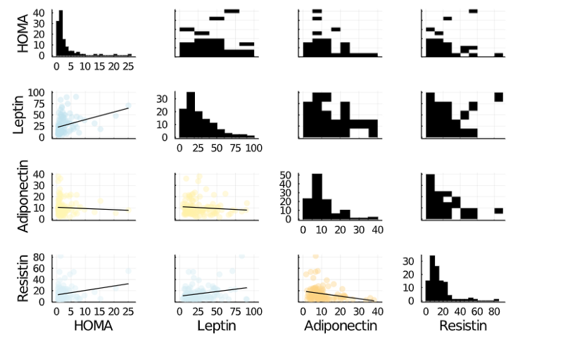
@df data corrplot(cols(1:4))
@df data corrplot(cols(5:8))
p=boxplot(layout=9,size=(1200,600))
for i in 1:9
    boxplot!(data_m[:,10],data_m[:,i] ,  group=data_m[:,10], subplot = i,title =names(data)[i] ,xaxis=nothing,label=["Control" "Patient"] )
end
display(p)
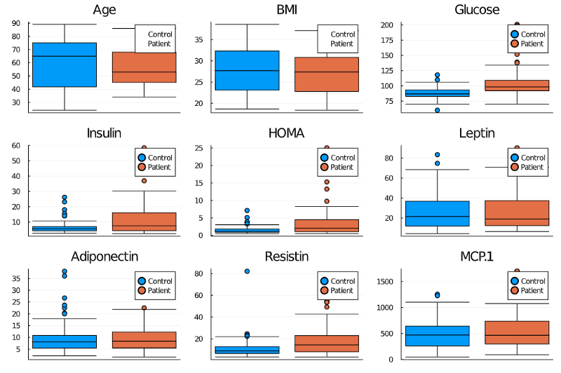
We can check with the graphs above that it really seems to be a difference in the classifiers regarding the target variable Classification. We can now make our models.
Creating Models
First, we unpack the data into a target (y) and predictors (X)
For getting more information on julia functions, we can type ??unpack to get more info.
y,X= unpack(data,==(:Classification),colname -> true);
MLJ provides the model function that has information on all the models that we can use. We can filter it by the data scitypes that we have (remember the coercing earlier).
models(matching(X, y)) #searching by input and target scitypes
We can also filter by name.
models("forest")#searching models by name
4-element Array{NamedTuple{(:name, :package_name, :is_supervised, :docstring, :hyperparameter_ranges, :hyperparameter_types, :hyperparameters, :implemented_methods, :is_pure_julia, :is_wrapper, :load_path, :package_license, :package_url, :package_uuid, :prediction_type, :supports_online, :supports_weights, :input_scitype, :target_scitype, :output_scitype),T} where T<:Tuple,1}: (name = RandomForestClassifier, package_name = DecisionTree, … ) (name = RandomForestClassifier, package_name = ScikitLearn, … ) (name = RandomForestRegressor, package_name = DecisionTree, … ) (name = RandomForestRegressor, package_name = ScikitLearn, … )
Let’s try and use a few models to get a better grasp of the package and existent models. Let’s try linear, non-linear and some more advanced models. But first, let’s create a training dataset and a test dataset and a dict to collect all the test results. rng is the seed for the randomization and guarantees reproducibility.
train, test = partition(eachindex(y), 0.8,shuffle=true,rng=42)
test_results=Dict();
For all the models, the workflow will be similar:
- load the model with @load
- create the machine according to our data (This does not train the model, only instantiates it).
- Fit and evaluate the performance of the model with the training dataset. In this case, we will use 10-fold cross-validation, collect two measures (accuracy and confusion matrix)Evaluate the performance of the model with the training dataset. In this case, we will use 10-fold cross-validation, and collect two measures (accuracy and confusion matrix).
- We then use the trained model to predict the unseen data (test set) and collect the accuracy in the test set in the previously created dictionary.
First, we can use the Linear Discriminant Analysis.
# LDA
Random.seed!(1234);
model_lda=@load LDA
mach_lda=machine(model_lda,X,y)
eval_lda=evaluate!(mach_lda, rows=train, resampling=CV(nfolds=10,shuffle=true,rng=42), measures=[accuracy,confusion_matrix],operation=predict_mode)
eval_lda.measurement[2]
ŷ = predict_mode(mach_lda, rows=test)
test_results["acc_lda"] = accuracy(ŷ, y[test])
For non-linear, we will try a decision tree and the k nearest neighbour algorithm (Knn).
# Decision tree
Random.seed!(1234);
model_tree = @load DecisionTreeClassifier
mach_tree = machine(model_tree, X, y)
eval_tree=evaluate!(mach_tree,rows=train, resampling=CV(nfolds=10,shuffle=true,rng=42), measures=[accuracy,confusion_matrix],operation=predict_mode)
eval_tree.measurement[2]
ŷ = predict_mode(mach_tree, rows=test)
test_results["acc_tree"] = accuracy(ŷ, y[test])
# KNN
Random.seed!(1234);
model_knn= @load KNNClassifier
mach_knn = machine(model_knn, X, y)
eval_knn=evaluate!(mach_knn, rows=train, resampling=CV(nfolds=10,shuffle=true,rng=42), measures=[accuracy,confusion_matrix],operation=predict_mode)
eval_knn.measurement[2]
ŷ = predict_mode(mach_knn, rows=test)
test_results["acc_knn"] =accuracy(ŷ, y[test])
Finally, we will try Support Vector Machines (SVM) and Random Forest (an ensemble of trees).
# SVM
model_svm= @load SVMLinearClassifier()
model_svm.random_state=1234 #you can easily modify models (here we add the random state)
mach_svm = machine(model_svm, X, y)
eval_svm=evaluate!(mach_svm,rows=train, resampling=CV(nfolds=10,shuffle=true,rng=42), measures=[accuracy,confusion_matrix],operation=predict)
eval_svm.measurement[2]
ŷ = predict(mach_svm, rows=test)
test_results["acc_svm"] = accuracy(ŷ, y[test])

# Random Forest
Random.seed!(1234);
model_rf= @load RandomForestClassifier pkg="DecisionTree"
mach_rf = machine(model_rf, X, y)
eval_rf=evaluate!(mach_rf, rows=train,resampling=CV(nfolds=10,shuffle=true,rng=42), measures=[accuracy,confusion_matrix],operation=predict_mode)
eval_rf.measurement[2]
ŷ = predict_mode(mach_rf, rows=test)
test_results["acc_rf"] = accuracy(ŷ, y[test])
Summing up
Now we collect all the accuracy calculated in the cross-validation and create a visualization presenting the average and standard deviations of the 10 results for each model.
results= [eval_lda.measurement[1], eval_knn.measurement[1],eval_svm.measurement[1],eval_rf.measurement[1],eval_tree.measurement[1]];
errors=[std(eval_lda.per_fold[1]),std(eval_knn.per_fold[1]),std(eval_svm.per_fold[1]),std(eval_rf.per_fold[1]),std(eval_tree.per_fold[1])]
scatter(["lda", "knn", "svm", "rf", "tree"],results,yerror=errors,ylims=[0,1],label="accuracy")

We can also check the accuracy of the test set.
scatter(Array(string.(keys(test_results))),Array(float.(values(test_results))),ylims=[0,1],label="accuracy")
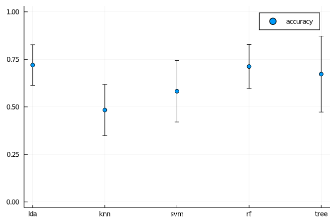
The best model for the test set seemed to be the decision tree. We can inspect the model further with these functions.
#checking fitting parameters for the possible best model
report(mach_lda)
fitted_params(mach_lda)
Conclusion
This was a simple exercise about how to use Julia and some more popular packages to create simple classification models.
We did not tune any of the models nor used any kind of hyperparameter modification. Nevertheless, we already could create models robust enough to make accurate predictions. Julia is a strong and robust language growing and very interesting to look into.
If you want to know more about Julia, check their website or their Github.
Happy coding! 🚀
(this post was collected from my medium profile)