Regression Tutorial with Julia lang

Hi, in my last post, I showed how Julia can be used to perform a classification task. In that case, we classified patients into two categories, so it was a classification, which is a method for predicting a, you guessed it, categorical outcome. But now, we are going to do a regression, where the outcome variable is continuous.

That said, let’s try to create a model that can predict the time to an event. Even though this could be handled differently, for this purpose, we are going to treat this outcome prediction as a simple continuous variable.

The dataset is available here. For this tutorial, we are going to need a few packages. For using them, check the code below.

If you do not have the packages installed, run

using Pkg; Pkd.add(“<PackageName>")

Data Load and Checking

For loading the dataset into your environment we can do it through the link. Then we should inspect the dataset in order to check if everything went as expected. Then we can analyse some descriptive statistics of the dataset, like central statistics and dispersion. We can sum all of this into:

For today, we are going to try to predict the variable time. This variable is the time to the event, which can be death or not. So time is the amount of time needed until that event, whether death or follow-up period. So we need to evaluate in detail the target variable with some visualizations.

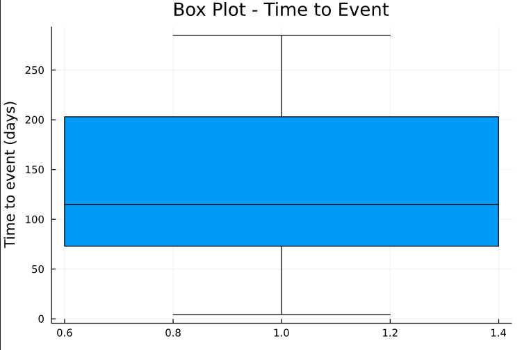
Time to the event has a median of +- 110 and an interquartile of 125. Now for a frequency plot.

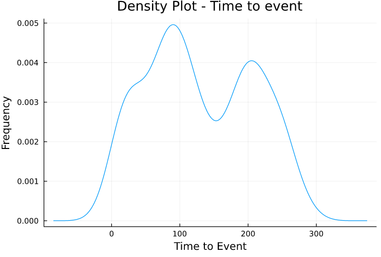
We have at least two peaks of time-frequency around 90 and 210.

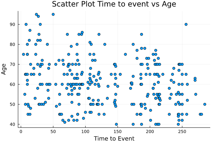
For a further inspection, we plotted age vs time. There is a negative correlation between them (even if low), as would be expected. Now for the event vs time.

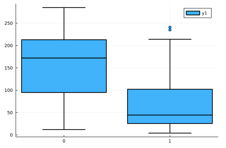
As expected, Event is a major differentiator for the value of time. So it will be natural that the variable event has a lot of impact on our model. Now to prepare the data for applying the models, we will coerce into specific scitypes for better handling by the models. More information on scitypes here.

coerce!(dataset, Count=>MLJ.Continuous);

Creating Models

Preparing data is important for starting the model creation, so we will divide data into target (y) and remaining features (X).

For this, we are going to evaluate the models in the training dataset with repeated cross-validation in order to get a pretty good idea of the model performance on the test set. For all models we are going to:

1. Load model.
2. Create the machine (which is a similar action to class instantiation)
3. Training with 3x 10-fold cross-validation and return the evaluation metric.
4. Store the metrics in a dictionary for further usage. So, we are going to use a linear model, decision tree, k-nearest neighbours, random forest and gradient boost (this could be done with a loop but oh well 😃). The seed is used to make the code reproducible (since RNG is used for cross-validation).

Assessing results

For the results, we need to collect all the Root Mean Squared Error returned by the cross-validations and evaluate the Confidence Interval (95%).

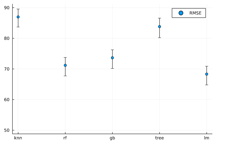
The Linear regression, Random Forest and GradientBoost seem to perform a little better than the other 2. However, since linear regression has a better explainability, we are going with it as the final model.

MAE: 51.26912864372159
RMSE: 59.80738088464344
RMSP: 2.398347880392765
MAPE: 0.9529914417765525

(coefs = [:age => -0.5600676786856139, :anaemia => -17.379451678818782, :creatinine_phosphokinase => -0.0024220637584861492, :diabetes => 5.5623104572596525, :ejection_fraction => -0.4719281676537811, :high_blood_pressure => -23.336061031579977, :platelets => -2.9328265873457684e-5, :serum_creatinine => 1.80232687559864, :serum_sodium => 0.06127126459720784, :sex => -3.8716177684193114, :smoking => -6.7752701233783705, :DEATH_EVENT => -86.69157019555797], intercept = 226.6056333198319,)

As we understood earlier, the DEATH_EVENT variable has a major impact in the model, with a -86 coefficient.

Evaluating Final Model

The model was fitted to the data and evaluated on the test set, we know how good it performed but we can investigate this more deeply. It should assess the errors for each row in the test set, in order to inspect them more thoroughly.

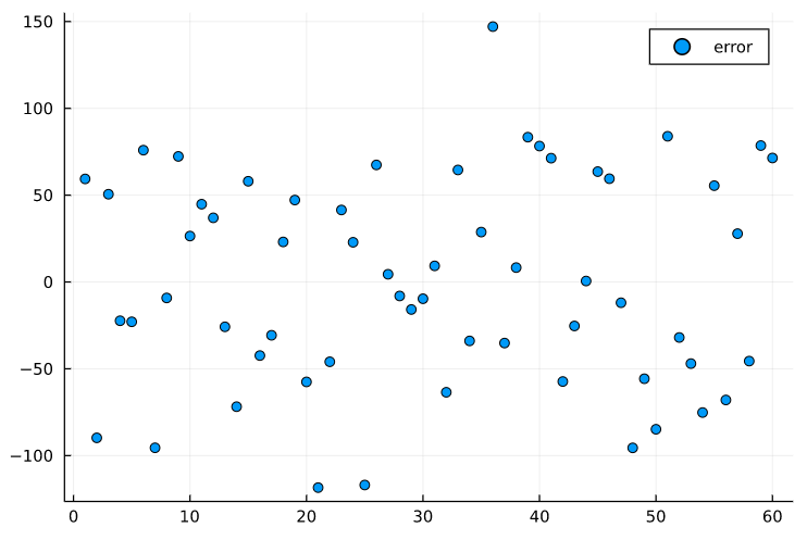
The errors seem random and do not follow any type of pattern, which is good.

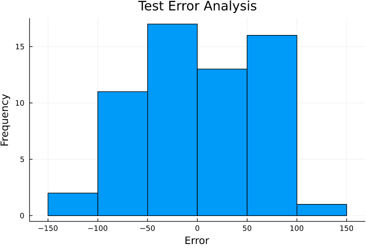
Test error seems to follow a normal distribution, which is desirable.

Conclusion

With these evaluations, we have a little more confidence to say that our model grasped a glimpse of the reality of the data in order to predict the time variable. Further work could be employed in tuning the parameters or creating variables to improve our models.

I hope that this was helpful to let you take on a regression task with Julia Lang!